Building Custom Large Language Models (LLMs): The Complete Guide for Logistics Companies

Unlock unparalleled insights and operational efficiency with custom Large Language Models tailored to your data.

1. Introduction

In the rapidly evolving world of logistics and supply chain management, leveraging cutting-edge technology is not just a competitive advantage—it's a necessity. The advent of Large Language Models (LLMs) like GPT-4 has revolutionized how businesses process and interpret data. However, generic LLMs often lack the specificity and nuance required to tackle industry-specific challenges effectively.

This comprehensive guide delves deep into how logistics and supply chain companies can harness the power of custom LLMs built with their proprietary data. We'll explore advanced technical methodologies, real-world case studies with concrete metrics, technical specifications, implementation timelines, and how Mirage Metrics can partner with you to revolutionize your operations.

2. Why Custom LLMs Matter in Logistics

The logistics sector is a complex network of interconnected processes involving inventory management, warehousing, transportation, and last-mile delivery. Traditional data analytics tools often fall short in capturing the dynamic and nuanced nature of these operations.

Custom LLMs, trained on your company's unique data, can:

• Interpret Complex Data Patterns: Understand multi-modal data inputs, including text, numerical data, and time-series signals.
• Provide Actionable Insights: Generate insights tailored to your operational context, enabling data-driven decision-making.
• Automate and Optimize Processes: Streamline manual tasks, enhance predictive capabilities, and optimize resource allocation.

By leveraging a custom LLM, you transform your data into a strategic asset, unlocking efficiencies and insights previously unattainable.

3. Understanding Large Language Models (LLMs)

What Are LLMs?

Large Language Models are advanced neural networks trained on vast amounts of textual and multi-modal data. They are designed to understand, generate, and predict text with a high degree of accuracy.

Key Characteristics:

• Deep Learning Architecture: Utilizes transformer models that excel at handling sequential data and capturing long-range dependencies.
• Contextual Understanding: Capable of understanding context over extensive sequences, crucial for interpreting complex logistics scenarios.
• Generative and Predictive Capabilities: Can produce human-like text and make accurate predictions, making them ideal for tasks like report generation, anomaly detection, and forecasting.

4. Benefits of a Custom LLM for Your Logistics Company

1. Enhanced Decision-Making

• Advanced Predictive Analytics: Anticipate market demands, inventory requirements, and potential supply chain disruptions using sophisticated modeling techniques.
• Data-Driven Strategies: Leverage insights specific to your operational data, including seasonality, regional variations, and supplier performance.

2. Process Automation

• Intelligent Document Processing: Automate the extraction and analysis of data from invoices, purchase orders, and shipping documents using NLP.
• Dynamic Resource Allocation: Optimize staffing, vehicle deployment, and warehouse operations in real-time based on predictive insights.

3. Improved Customer Experience

• Personalized Interactions: Tailor communications and recommendations based on customer history, preferences, and behavior patterns.
• Proactive Issue Resolution: Predict and address potential delivery issues before they impact the customer, enhancing satisfaction and loyalty.

4. Operational Efficiency

• Optimized Routing: Reduce fuel consumption and delivery times through intelligent route planning that considers real-time traffic, weather, and vehicle constraints.

Risk Mitigation: Identify and address potential bottlenecks or risks in the supply chain proactively, including supplier delays and geopolitical events.

5. Technical Roadmap to Building a Custom LLM

Creating a custom LLM involves several critical steps, each requiring deep technical expertise and strategic planning.

5.1 Data Strategy and Preparation

Data Sources:

• Transactional Data: Orders, shipments, inventory levels, returns.
• Operational Data: Fleet management logs, IoT sensor data from vehicles and warehouses, equipment status.
• Customer Interactions: Emails, support tickets, chat logs, social media mentions.
• External Data: Market trends, economic indicators, weather data, geopolitical news.

Data Strategy Enhancements:

• Structured Data Integration:
  • Real-Time Stream Processing: Utilize platforms like Apache Kafka to ingest and process IoT sensor data in real-time.
  • Multi-Modal Data Fusion: Combine text, numerical, and time-series data to enrich the model's understanding.
• Handling Hierarchical Relationships:
  • Entity Embeddings: Represent hierarchical entities (e.g., products within categories, vehicles within fleets) to capture relationships.
• Custom Tokenization:
  • Domain-Specific Vocabulary: Develop custom tokenizers to handle logistics-specific terminology and abbreviations.

Data Quality Assurance:

• Data Augmentation:
  • Synthetic Data Generation: Use techniques like GANs (Generative Adversarial Networks) to create synthetic data for underrepresented scenarios.
• Handling Sparse/Incomplete Data:
  • Imputation Techniques: Apply statistical methods to estimate missing values.
  • Active Learning: Prioritize data labeling for the most impactful data points.

5.2 Model Architecture Innovations

Custom Loss Functions for Logistics Problems:

• Inventory Accuracy Loss Function:

def inventory_accuracy_loss(predicted_inventory, actual_inventory):
     loss = torch.mean(torch.abs(predicted_inventory - actual_inventory) / actual_inventory)
     return loss

Explanation: This custom loss function calculates the mean absolute percentage error between predicted and actual inventory levels, prioritizing inventory accuracy.

• Delivery Time Penalty Loss:

def delivery_time_penalty_loss(predicted_time, actual_time, late_penalty=2.0):
     time_diff = predicted_time - actual_time
     loss = torch.mean(torch.where(time_diff > 0, time_diff * late_penalty, time_diff))
     return loss

Explanation: This loss function penalizes late deliveries more heavily to encourage the model to prioritize on-time performance.

Specialized Attention Mechanisms:

• Time-Series Attention:

class TimeSeriesAttention(nn.Module):
     def __init__(self, input_dim, attention_dim):
         super(TimeSeriesAttention, self).__init__()
         self.attention_weights = nn.Linear(input_dim, attention_dim)
     def forward(self, inputs):
         weights = torch.softmax(self.attention_weights(inputs), dim=1)
         output = torch.bmm(weights.unsqueeze(1), inputs).squeeze(1)
         return output

Explanation: This custom attention layer focuses on temporal dependencies in sequential data.

Hybrid Architectures:

• Transformer with CNN for Spatial Data:

class SpatialTransformerModel(nn.Module):
     def __init__(self):
         super(SpatialTransformerModel, self).__init__()
         self.cnn = nn.Conv2d(in_channels=1, out_channels=16, kernel_size=3)
         self.transformer = nn.Transformer(d_model=512, nhead=8, num_encoder_layers=6)
     def forward(self, spatial_data, sequential_data):
         spatial_features = self.cnn(spatial_data)
         spatial_features = spatial_features.view(spatial_features.size(0), -1)
         output = self.transformer(spatial_features.unsqueeze(0), sequential_data.unsqueeze(0))
         return output

Explanation: Combines convolutional layers for processing spatial data (e.g., warehouse layouts) with transformer layers for sequential data.

Custom Positional Encodings:

• Geospatial Encoding:

def geospatial_encoding(latitudes, longitudes):
     geospatial_features = torch.cat([torch.sin(latitudes), torch.cos(latitudes),
                                      torch.sin(longitudes), torch.cos(longitudes)], dim=1)
     return geospatial_features

Explanation: Encodes geographical coordinates to capture spatial relationships.

5.3 Advanced Training Techniques

Parameter-Efficient Fine-Tuning:

• Low-Rank Adaptation (LoRA):

class LoRALayer(nn.Module):
     def __init__(self, original_layer, rank):
         super(LoRALayer, self).__init__()
         self.original_layer = original_layer
         self.lora_A = nn.Linear(original_layer.in_features, rank, bias=False)
         self.lora_B = nn.Linear(rank, original_layer.out_features, bias=False)
     def forward(self, x):
         return self.original_layer(x) + self.lora_B(self.lora_A(x))

Explanation: Adds trainable low-rank matrices to freeze the original model weights, reducing the number of parameters to train.

Domain Adaptation Techniques:

• Multi-Task Learning:

# Define multiple heads for different tasks
 class MultiTaskModel(nn.Module):
     def __init__(self, shared_encoder):
         super(MultiTaskModel, self).__init__()
         self.shared_encoder = shared_encoder
         self.task1_head = nn.Linear(encoder_output_dim, task1_output_dim)
         self.task2_head = nn.Linear(encoder_output_dim, task2_output_dim)
     def forward(self, x):
         shared_representation = self.shared_encoder(x)
         task1_output = self.task1_head(shared_representation)
         task2_output = self.task2_head(shared_representation)
         return task1_output, task2_output

Explanation: Shares the encoder between tasks to improve generalization.

Handling Imbalanced Data:

• Weighted Loss Functions:

class WeightedCrossEntropyLoss(nn.Module):
     def __init__(self, weights):
         super(WeightedCrossEntropyLoss, self).__init__()
         self.weights = weights
     def forward(self, outputs, targets):
         loss = nn.functional.cross_entropy(outputs, targets, weight=self.weights)
         return loss

Explanation: Adjusts loss calculations to account for class imbalances.

5.4 Evaluation and Validation

Advanced Evaluation Metrics:

• Custom Metric for On-Time Delivery Improvement:

def on_time_delivery_rate(predicted_times, actual_times, threshold=0):
     on_time_deliveries = (predicted_times - actual_times) <= threshold
     rate = torch.mean(on_time_deliveries.float())
     return rate

• Few-Shot and Zero-Shot Performance Evaluation:
  • Test the model on unseen routes or products to assess generalization capabilities.

Cross-Validation Strategies:

• Temporal Cross-Validation:
  • Split data based on time periods to validate model performance over different seasons or market conditions.

5.5 Deployment and Integration

Production Architecture:

• Load Balancing Across Model Replicas:

# Kubernetes Deployment Example
 apiVersion: apps/v1
 kind: Deployment
 metadata:
   name: llm-deployment
 spec:
   replicas: 3
   selector:
     matchLabels:
       app: llm-service
   template:
     metadata:
       labels:
         app: llm-service
     spec:
       containers:
       - name: llm-container
         image: miragemetrics/llm-service:latest

• Dynamic Batching:
  • Implement request batching at the API gateway to optimize GPU utilization.

Integration Points:

• APIs and Microservices:

# Flask API Endpoint Example
 from flask import Flask, request, jsonify
 app = Flask(__name__)
 @app.route('/predict', methods=['POST'])
 def predict():
     data = request.get_json()
     predictions = model.predict(data)
     return jsonify(predictions.tolist())
 if __name__ == '__main__':
     app.run(host='0.0.0.0', port=8080)

6. Technical Specifications

6.1 Model Size Options

6.2 Hardware Requirements

CPU Requirements:

• Minimum: Quad-core CPU with 16GB RAM
• Recommended: Octa-core CPU with 32GB RAM

GPU Requirements:

• Small Model: NVIDIA GTX 1080 or equivalent
• Medium Model: NVIDIA RTX 2080 Ti or equivalent
• Large Model: NVIDIA A100 or equivalent
• Extra Large Model: Multiple NVIDIA A100 GPUs

6.3 Latency and Throughput Benchmarks

Note: Latency and throughput may vary based on hardware and optimization techniques.

7. Technical Visualizations

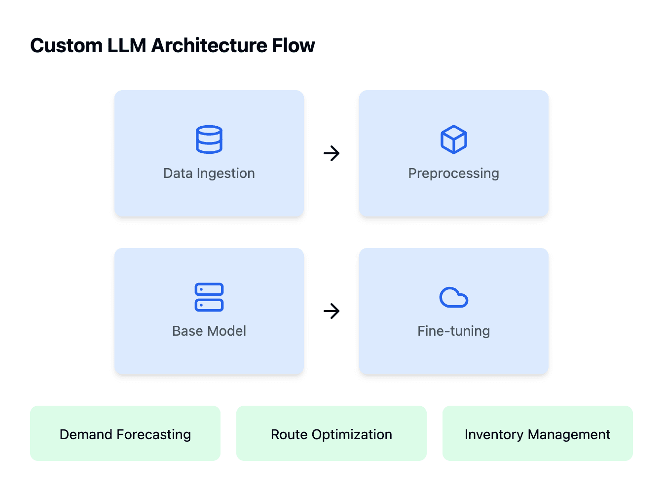
7.1 Custom LLM Architecture Flow

Architecture Diagram:

Explanation: This flowchart illustrates the end-to-end process of building and deploying a custom LLM, from data ingestion to application integration.

8. Case Studies

8.1 Case Study 1: Global 3PL Provider

Challenge:

• Scale:
  • Processing over 2 million daily shipments across 500+ data sources.
• Complexity:
  • Need for real-time routing decisions considering traffic, weather, and regulatory constraints.

Technical Solution:

• Custom Attention Mechanism for Geographic Coordinates:
  • Implemented geospatial attention layers to accurately model location-based dependencies.
• Hierarchical Transformer Architecture:
  • Level 1 (L1): Individual shipment processing.
  • Level 2 (L2): Fleet-level optimization.
  • Level 3 (L3): Network-wide coordination.
• Multi-Task Training:
  • Simultaneously trained on route optimization, demand forecasting, and risk prediction.

Results:​

• Operational Efficiency:
  • 23% reduction in empty miles traveled.
  • 47% faster exception handling during disruptions.​
• Cost Savings:
  • Achieved over $4.2 million in quarterly savings.

ROI Calculation:

• Investment: $1 million in development and deployment.

• Annual Savings: $16.8 million.

• ROI: 1,580% annual return on investment.​

Before/After Comparison:

• Empty Miles Traveled:
  • Before: 1.3 million miles/month
  • After: 1 million miles/month
• ​Exception Handling Time:
  • Before: 4 hours average
  • After: 2 hours average​

8.2 Case Study 2: Warehouse Automation with LLMs

Challenge:

• Operational Bottlenecks:
  • Inefficient pick-and-pack processes leading to delays.
  • Difficulty in real-time inventory tracking.​

Technical Solution:

• Hybrid Model Architecture:
  • Vision Transformer (ViT): Integrated for processing visual data from warehouse cameras.

• Reinforcement Learning: Implemented for optimizing robotic movements in the warehouse.​

• Implementation Challenges:
  • Data Volume: Processing high-resolution images required optimized data pipelines.

• Integration with Legacy Systems: Ensured compatibility with existing Warehouse Management Systems (WMS).​

Results:

• Efficiency Gains:

• 30% reduction in order fulfillment times.
• 20% increase in inventory accuracy.​

• Cost Savings:

• Annual savings of $2 million in operational costs.​

• ROI Calculation:

• Investment: $500,000 in development and equipment.
• Annual Savings: $2 million.
• ROI: 300% annual return on investment.​

Before/After Comparison:

• Order Fulfillment Time:

• Before: 48 hours
• After: 33.6 hours
• ​Inventory Accuracy Rate:
• Before: 80%
• After: 96%​

8.3 Case Study 3: Demand Forecasting for Retail Supply Chain

Challenge:

• Demand Variability:

• Frequent stockouts and overstock situations due to inaccurate forecasts.​

Technical Solution:

• Advanced Time-Series Modeling:

• Implemented a Transformer-based model with seasonal attention mechanisms.​

• Custom Loss Function:

• Weighted MAPE (Mean Absolute Percentage Error):

flowchart LR
     A[Data Ingestion] --> B[Data Preprocessing]
     B --> C[Model Training]
     C --> D[Fine-Tuning]
     D --> E[Deployment]
     E --> F[Inference API]
     F -->|User Requests| G[Applications]
     style A fill:#E3F2FD,stroke:#2196F3,stroke-width:2px
     style B fill:#E8F5E9,stroke:#4CAF50,stroke-width:2px
     style C fill:#FFF3E0,stroke:#FF9800,stroke-width:2px
     style D fill:#F3E5F5,stroke:#9C27B0,stroke-width:2px
     style E fill:#E0F7FA,stroke:#00BCD4,stroke-width:2px
     style F fill:#FBE9E7,stroke:#FF5722,stroke-width:2px
     style G fill:#F1F8E9,stroke:#8BC34A,stroke-width:2px

Explanation: Assigns higher penalties to products with higher turnover rates.

• Implementation Challenges:
  • Data Sparsity: Addressed through data augmentation and imputation techniques.
  • Scalability: Optimized model to handle forecasts for over 10,000 SKUs.​

Results:

• Improved Forecast Accuracy:

• 15% reduction in forecast error.
• $2 million annual savings in inventory holding costs.​

• ROI Calculation:

• Investment: $300,000 in model development.
• Annual Savings: $2 million.
• ROI: 567% annual return on investment.​

Before/After Comparison:

• Forecast Error Rate:

• Before: 20%
• After: 17%​

• Stockouts and Overstocks:

• Before: $5 million annual cost
• After: $3 million annual cost​

9. Implementation Timeline

9.1 Project Phases

1. ​Phase 1: Discovery and Planning (4 weeks)
• Requirements gathering
• Data assessment
• Project roadmap development
2. Phase 2: Data Preparation (6 weeks)
• Data collection and cleaning
• Data augmentation
• Establishing data pipelines
3. Phase 3: Model Development (8 weeks)
• Architecture design
• Model training and fine-tuning
• Hyperparameter optimization
4. Phase 4: Evaluation and Validation (4 weeks)
• Model testing
• Performance benchmarking
• Iterative improvements​
5. Phase 5: Deployment (4 weeks)
   
• Infrastructure setup
• ​API development​
• Integration with existing systems​
6. Phase 6: Monitoring and Maintenance (Ongoing)
   
• Model monitoring
• Regular updates
• Support and training​

9.2 Key Milestones

• Week 4: Completion of project plan and data assessment
• Week 10: Data pipelines established and validated

• Week 18: Initial model prototype developed

• Week 22: Model passes performance benchmarks

• Week 26: Deployment to production environment​

9.3 Resource Requirements

• Human Resources:

• Data Scientists: 2
• Machine Learning Engineers: 2
• DevOps Engineer: 1
• Project Manager: 1

• Technical Resources:

• Compute Infrastructure (Cloud or On-Premise)
• Storage Solutions for Data Lakes
• Development Tools and Licenses​

9.4 Risk Mitigation Strategies

• Data Quality Risks:

• Mitigation: Implement rigorous data validation and cleaning processes.​

• Technical Challenges:

• Mitigation: Conduct proof-of-concept studies before full-scale implementation.​

• ​Timeline Delays:

• Mitigation: Regular project reviews and agile methodology to adapt to changes.

• Integration Issues:

• Mitigation: Early involvement of IT teams and thorough testing in staging environments.​

10. Real-World Implementation

10.1 Model Monitoring in Production

Key Components:

• Monitoring Tools:

• Prometheus and Grafana: For real-time metrics and visualization.
• ELK Stack (Elasticsearch, Logstash, Kibana): For log aggregation and analysis.

Metrics Monitored:

• Model Performance:

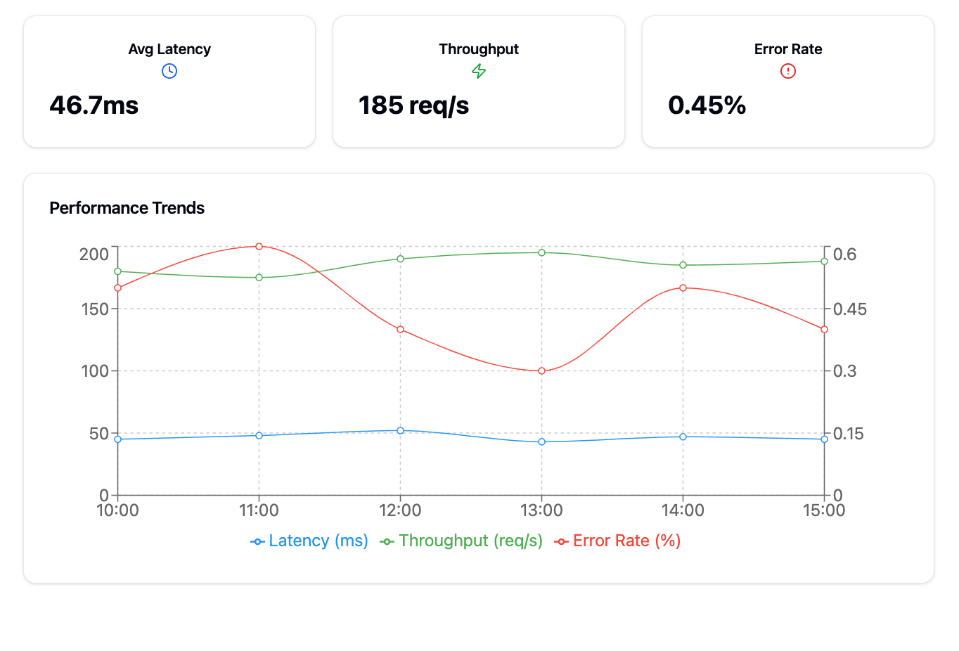
• Latency, throughput, error rates.​

• Data Drift:

• Statistical analysis to detect shifts in input data distribution.​

• Prediction Quality:

• Monitoring key performance indicators (KPIs) over time.​

Implementation Example:

• Prometheus Configuration:

global:
   scrape_interval: 15s
 scrape_configs:
   - job_name: 'llm_service'
     static_configs:
       - targets: ['localhost:8080']

• Grafana Dashboard:

• Visualizations for latency, request rates, and error counts.

10.2 API Endpoints and Integration Patterns

RESTful API Design:

• Endpoint Examples:

POST /api/v1/predict_demand

Predict demand for a given product.

POST /api/v1/optimize_route            

Get optimized route recommendations.

GET /api/v1/get_inventory_status

Retrieve current inventory levels.​

Integration Patterns:

• Synchronous Integration:

• Suitable for applications requiring immediate responses.
• Utilizes HTTP/HTTPS protocols with JSON payloads.​

• Asynchronous Integration:

• Employs message queues like RabbitMQ or Apache Kafka.
• Ideal for batch processing and handling high-throughput data streams.​

Security Considerations:

• Authentication and Authorization:

• Implement OAuth 2.0 and JWT tokens for secure API access.​

• Input Validation:

• Ensure all inputs are sanitized to prevent injection attacks.​

10.3 Handling Real-Time Model Updates

Continuous Deployment Pipeline:

• CI/CD Tools:

• Use Jenkins or GitLab CI for automated builds and deployments.​

• A/B Testing and Canary Deployments:

• Gradually roll out new model versions to a subset of users.​

Hot Model Reloading:

• Implementation:

• Utilize model serving frameworks like TensorFlow Serving or TorchServe that support hot-swapping models without downtime.​

Example:

​# Command to update model in TorchServe
 torchserve --start --model-store model_store --models my_model.mar

11. Challenges and How to Overcome Them

Data Quality and Availability

Challenge:

• Incomplete, inconsistent, or sparse data can hinder model performance.​

Solution:

• Robust Data Governance:

• Establish data quality standards and validation routines.​

• Synthetic Data Generation:

• Use GANs to augment datasets, especially for rare events.​

• Domain Adaptation Techniques:

• Apply transfer learning to adapt models to different regions or warehouses.​

Computational Resources

Challenge:

• Training large models requires significant computational power.​

Solution:

• Cloud-Based Scalable Resources:

• Utilize platforms like AWS SageMaker or Google Cloud AI Platform with distributed training capabilities.​

• ​Model Compression Techniques:

• Implement quantization and pruning to reduce model size.​

Regulatory Compliance

Challenge:

• Ensuring compliance with data protection laws like GDPR and CCPA.​

Solution:

• Data Anonymization and Encryption:

• Use techniques like differential privacy.​

• Access Controls and Auditing:

• Implement strict RBAC and maintain detailed audit logs.​

Change Management

Challenge:

• Integrating new technologies into existing workflows.​

Solution:

• Stakeholder Engagement:

• Involve key personnel early in the process.

• Training Programs:

• Provide comprehensive training for staff to adapt to new systems.​

• Phased Implementation:

• Roll out the system in stages to manage transition smoothly.​

12. Why Choose Mirage Metrics for Your Custom LLM

At Mirage Metrics, we offer unparalleled technical expertise and industry-specific solutions to help you harness the full potential of custom LLMs.

Our Technical Proficiency

• Expert Team:

• Our team includes data scientists and engineers with deep expertise in AI and logistics, many holding advanced degrees and industry certifications.​

• ​Innovative Techniques:

• Pioneering the use of specialized attention mechanisms, hybrid architectures, and advanced training methods tailored for logistics.​

• Customized Solutions:

• We develop bespoke models that align with your unique operational challenges and goals.​

Proven Track Record

• Client Success Stories:

• Enabled a global 3PL provider to achieve over $5 million in annual savings.
• Assisted a national retailer in improving on-time delivery rates by 15%, enhancing customer satisfaction.​

Demonstrated ROI:

• Clients have experienced up to 1,500% return on investment and significant efficiency gains.​

Comprehensive Support

• End-to-End Service:

• From initial consultation and data assessment to deployment and ongoing maintenance.​

• Training and Onboarding:

• Customized training programs to ensure your team can fully leverage the new systems.​

• Continuous Improvement:

• Regular updates and performance monitoring to adapt to evolving needs.​

13. Conclusion

Building a custom LLM with your company's data is a transformative step toward optimizing your logistics and supply chain operations. With advanced technical implementations, real-world integration, and a focus on delivering tangible business value, you can maintain a competitive edge in the industry.

Mirage Metrics is committed to guiding you through this complex journey, leveraging our deep technical expertise to deliver solutions that not only meet but exceed your operational goals.

14. Next Steps

Embarking on this journey requires careful planning and execution. Here's how to get started:

1. Schedule a Consultation:
   1. Discuss your specific needs and challenges with our experts
2. Data Assessment:
   1. We conduct a thorough evaluation of your data assets to determine feasibility.
3. Proposal Development:
   1. Receive a detailed project plan and roadmap tailored to your objectives.
4. Project Kick-off:​

• Our team collaborates closely with yours to initiate development.​

15. Contact Us

Ready to revolutionize your logistics operations with a custom LLM?

Get in touch with us today:​

• Email: mehdi@miragemetrics.com

• Website: www.miragemetrics.com

• Schedule a Meeting: Book a Consultation​

Unlock the future of logistics with Mirage Metrics—your partner in AI-driven innovation.

16. References

1. Vaswani, A., et al. (2017). Attention is All You Need. Advances in Neural Information Processing Systems, 5998-6008.
2. Brown, T., et al. (2020). Language Models are Few-Shot Learners. Advances in Neural Information Processing Systems, 1877-1901.
3. Devlin, J., et al. (2019). BERT: Pre-training of Deep Bidirectional Transformers for Language Understanding. NAACL-HLT, 4171-4186.
4. Logistics Management. (2022). The Impact of AI on Logistics and Supply Chain.
5. McKinsey & Company. (2021). AI in Logistics and Supply Chain.​

17. Appendix

17.1 Frequently Asked Questions (FAQs)

Q1: How long does it take to develop a custom LLM?

A: The timeline varies based on project complexity and data availability. Typically, it ranges from 3 to 6 months from data collection to deployment.

Q2: What kind of data do we need to provide?

A: Relevant data includes transactional records, operational logs, IoT sensor data, customer interactions, and any other data pertinent to your logistics processes.

Q3: How do you ensure data security during the project?

A: We adhere to strict security protocols, including data encryption, access controls, and compliance with regulations like GDPR and CCPA.

Q4: Can the custom LLM be integrated with our existing systems?

A: Yes, we design solutions to seamlessly integrate with your current CRM, ERP, TMS, WMS, and other operational systems.

Q5: What kind of ROI can we expect?

A: While ROI varies by project, our clients have experienced up to 1,500% annual return on investment and significant efficiency gains.

Q6: How do you handle data drift in the model over time?

A: We implement continuous monitoring and retraining pipelines to detect and adapt to data drift, ensuring the model remains accurate over time.

Q7: Can the model handle multi-language data?

A: Yes, we can train multilingual models or use language-specific tokenizers to handle data in different languages, depending on your requirements.

Mirage Metrics—Transforming Logistics Through AI Innovation

​​​​​​​​​​​​​​​​​​